Using Tracealyzer to Evaluate Python Algorithms in Linux

Mohammed Billoo, founder of MAB Labs (www.mab-labs.com), provides custom embedded Linux solutions for a multitude of hardware platforms. In a series of posts he walks us through the Linux support in Tracealyzer v4.4.

In a previous post we discussed how we can use Tracealyzer to evaluate user space applications on a Linux-based embedded system. In that example, we emulated a potential feature and wished to evaluate the performance of multiple implementation candidates. We learned the necessary function invocations in our C/C++ application to trigger tracepoints, which would serve as markers in our Tracealyzer timeline. We also learned the necessary configuration in Tracealyzer to convert the tracepoints into “Custom Intervals”, which are ultimately used to provide us with the necessary timing information to evaluate the various implementations.

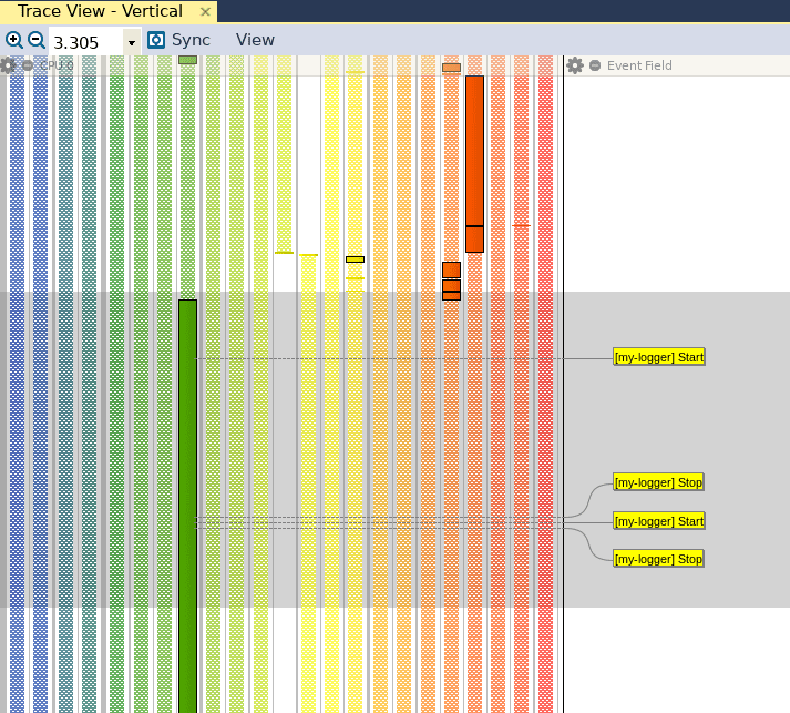
In this blog post, we will see how Tracealyzer can be used to quickly and efficiently evaluate multiple implementations of an algorithm in Python. Due to the increased desire to perform machine learning at the “edge”, Python is becoming more common in embedded application development; most machine learning frameworks are implemented in Python.

How (not) to compute Fibonacci numbers

As mentioned, we’re going to walk through a simple example and discover an interesting caveat of application development in Python. This example will also demonstrate how the combination of LTTng and Tracealyzer can be used to efficiently compare the performance of two implementations of the same algorithm.

Specifically, we’re going to implement the Fibonacci sequence using two common techniques. The first technique is to use a recursive algorithm, and the second technique is to use a standard iterative algorithm. We will then use LTTng and Tracealyzer to compare the performance of these two techniques.

However, before we begin, we need to ensure that the Python LTTng software package is installed. Additional details on how to install the necessary software package can be found on LTTng’s website here: https://lttng.org/docs/v2.12/#doc-ubuntu.

We will start with both implementations of the Fibonacci sequence, which will be done in a single module:

def recur_fibo(n):
  if n <=1 n:
    return n
  else:
    return(recur_fibo(n-1) + recur_fibo(n-2))

def non_recur_fibo(n):
  result = []
  a,b = 0,1
  while a < n:
    result.append(a)
    a,b = b, a+b
  return result

We would then have our separate Python source file that calls the two functions above, with some key lines that are in bold (which we’ll discuss later):

import lttngust
import logging
import fib

def example():
  logging.basicConfig()
  logger = logging.getLogger(‘my-logger’)
  logger.info(‘Start’)
  fib.recur_fibo(10)
  logger.info(‘Stop’)
  logger.info(‘Start’)
  fib.non_recur_fibo(10)
  logger.info(‘Stop’)

if __name__ == ‘__main__’:
  example()

Then, we execute the following commands to capture a trace for consumption in Tracealyzer:

$> lttng create
$> lttng enable-event --kernel sched_switch
$> lttng enable-event --python my-logger
$> lttng start
$> python3 <example source file>.py
$> lttng stop
$> lttng destroy

In the above snippet, the command in bold is key. Here we are replacing the standard Python logger with one called “my-logger”, and storing these events in the resulting LTTng trace. The lines in bold in the Python snippet above establish this “my-logger” logger and emit the events surrounding our test functions. The actual severity of the logs can be anything, since they will be ignored. We can see that the mechanism used to emit events to mark function boundaries is similar to that seen in the previous post.

Once the trace has been generated, we can open it in Tracealyzer and see that our events appear in the Trace View:

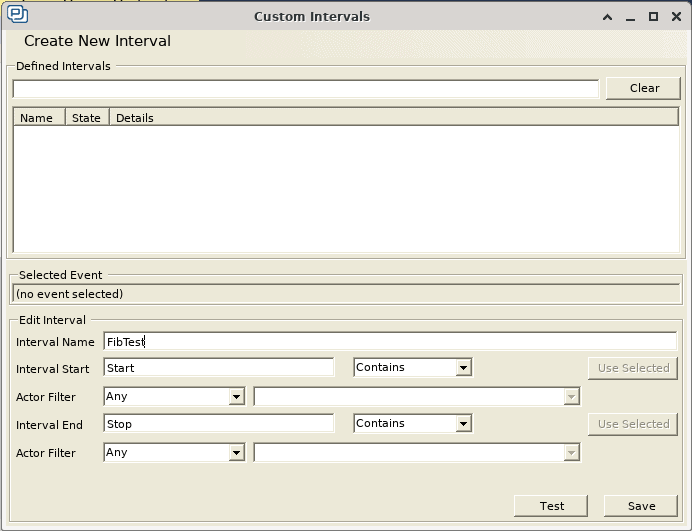
Since we are not capturing any data in this particular example, we don’t need to configure event interpretations to read the data values. All we need to do is create a Custom Interval to mark the entry and exit of both of these functions. While we can already see that there is a substantial performance difference in the Trace View above, we’d like to retrieve more tangible performance metrics. As mentioned in a previous post, this can be done by going to Views, and clicking on Intervals and State Machines. Then, we can click on Custom Intervals, and create the following custom interval:

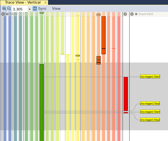
We have used the strings “Start” and “Stop” to mark the entry and exit of our candidate functions, so we will use these two strings to mark the start and stop of our custom interval. When we click on Save, we can see that the Trace View has been updated with a new red bar to the right, which identifies our custom interval:

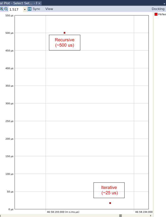
When we open the Interval Plot by clicking on Views and then on Interval Plot – Select Set… and adjust the view in the resulting graph to show no lines, we can see that there is a 20x difference in performance between the recursive algorithm (which was executed first) and the iterative algorithm (which was executed second).

We have quickly discovered that recursion is inherently slow in Python! If we go back to our Python implementation, we only ran 10 iterations of each algorithm. If we didn’t have Tracealyzer, we would need to run many more iterations to gain some meaningful insight. However, this approach is problematic for two reasons. First, if you run the recursive algorithm with 1000 (or even 100) iterations, Python will simply sit there (try it!). This would be concerning to us as developers, since we don’t know whether this tremendous slow down is due to a bug in our implementation or something else entirely.

This question becomes more relevant as the algorithm or implementation becomes more complex, as more substantive logging will be required to understand where the bottleneck is. Second, if there are multiple applications running on our deployed embedded system, these other applications could be disrupting our own application and increasing the time for our algorithm or function to complete execution. Without a trace, we would not be able to tell if this was the case.

Tracepoints incur minimal overhead

Instead, the combination of LTTng in Python and Tracealyzer has allowed us to discover a fundamental characteristic of the Python language that would be invaluable to us as we develop more complex algorithms. Since tracepoints add minimal overhead, we can keep them in our application as we test it on our target embedded system. This will allow us to gain insights into the performance of our application while other applications are running.

Our implementation above also serves as a reference on how the performance of future algorithm implementations can be evaluated. As shown above, we have isolated the core functions themselves into a separate Python module. Not only is this good programming practice in general, but this lets us focus on the performance of specific functions. Just as we created a more encompassing Python module that made direct calls to the core functions, we would create a series of “test” modules that would emit similar events before making calls to the functions under test.

Additionally, since trace overhead is almost negligible, we can actually generate performance metrics in our production codebase as well. This would be tremendously useful for regular system testing, wherein the same codebase can be used to ensure that the application is both functionally correct and performant, with only minimal changes.

Conclusions

In summary, we have demonstrated how we can use Tracealyzer and LTTng to capture performance metrics in a Python application. Due to its minimal overhead, we can retain the instrumentation for use on our target embedded system, which allows us to monitor and understand the interaction that our application has with other applications and the operating system as well. For example, there may be another process or thread that may preempt our application and hinder the performance of our application. We can use Tracealyzer and LTTng to understand the cause of such performance anomalies and refine our implementation to guard against them.

Additionally, by using a relatively innocuous example, we’ve learned a key characteristic of the Python language that we can use in future, more complex implementations. We’ve also shown an appropriate design to measure and validate the performance of key core functions that may be kept relatively isolated. Finally, we’ve demonstrated how this mechanism can be expanded to ensure that our application is functionally correct and performant with minimal changes in our environment and setup.

03-06-2021